Here is the uncomfortable truth that most camera trap survey design comes down to: spacing, density, and duration are not three independent dials you tune to taste. They are all downstream of one decision you make before a single camera leaves the truck — what, exactly, are you trying to estimate? Species richness, occupancy, relative abundance, and density each demand a different array, a different number of stations, and a different length of deployment, and a design that's excellent for one can be quietly useless for another.
That sounds obvious. It clearly isn't. When Burton and colleagues reviewed 266 camera trap studies published between 2008 and 2013, 40.2% did not use a probability-based sampling design at all, relying on opportunistic or targeted placement, and a further 21.4% gave almost no details on sampling design. Fewer than a third explicitly mentioned the assumptions of spatial and temporal independence their analyses depended on. The cameras worked fine. The designs, in many cases, could not support the inferences the authors drew from them.
So before we get to numbers — and there are good, specific numbers below — internalize the order of operations. Pick the question. Let the question set the spacing relative to your target species' home range. Let spacing and your precision target set the number of stations. Let detectability set the duration. Everything else is logistics. Get the order wrong and no amount of field effort will save you.
Start with the question, not the camera
The single most useful framing in the literature is that a camera detection is the product of two processes: how many animals are out there, and how likely each one is to be photographed. Every design choice is really a choice about how you handle that second process — detection. What separates the analytical methods is what they assume, and therefore what they require of your array.
A quick tour of the four common goals, because the rest of this article keeps referring back to them:
- Species inventory / richness — "what lives here?" You need every species to have a non-zero chance of detection, which mostly means broad spatial coverage and randomization, not intensity at any one spot.
- Occupancy — "what proportion of sites is a species using?" The occupancy framework explicitly models imperfect detection through repeat visits, so it needs enough sites and enough survey occasions per site to pin down detection probability.
- Relative abundance (RAI) — detections per unit effort, used as an index of abundance. Cheap and ubiquitous, but it rests on the heroic assumption that detectability is constant across the things you're comparing. It usually isn't.
- Density — animals per unit area, the gold standard. For individually identifiable species (think spotted cats) this means spatial capture–recapture (SCR/SECR); for unmarked species, the random encounter model (REM) is the main game in town. These two methods want opposite things from your camera spacing, which is the single biggest trap in the whole field.
The GBIF data-publishing guide makes the same point from the other end: "what would you like to know from which species groups? Each aim brings along its own key characteristics to consider, such as camera height and direction, seasonality, bait usage, detection zone features". Those characteristics aren't optional metadata. They're the design.
A practitioner's overview that's worth a beginner's time frames placement itself as a menu — random, stratified, systematic, adaptive, and occupancy-style sampling, each with its own strengths. That's a fine mental scaffold. But the moment you're choosing real coordinates, the question is no longer "which sampling archetype sounds good" — it's "what does my estimator assume, and does this layout satisfy it?"
Spacing and independence: tied to home range, not habit
Camera spacing is where good intentions go to die, because the "right" spacing flips depending on your goal — and the literature genuinely disagrees in places, which I'll flag as we go.
For richness, occupancy, and RAI, you generally want independence. The rule of thumb almost everyone reaches for is 1–2 km between stations. That number isn't sacred; it's a pragmatic stand-in for "far enough apart that two cameras aren't sampling the same individuals." The WWF best-practices guide is blunt that the importance of strict independence "is often overstated, and may have little effect on statistical inference," noting that the spatial clumping you'd worry about has been found to be weak in camera data when anyone looked for it. Kays and colleagues found autocorrelation between cameras wasn't an issue beyond about 25 m in tropical forest — but a subtropical scrub study still found it at 500 m. So the honest version: tie spacing to the home-range size of your target species, default to roughly 1 km (and at least one home-range diameter) when you lack that information, and remember you can model residual dependence statistically rather than design it away.
WildCAM's setup guide gives the cleanest plain-language version of the trade-off: if you're estimating grizzly bear occupancy "and cameras are placed too close together, detections may not be statistically independent if there's a chance that the same individual is detected at neighbouring camera sites within a short period of time," so for wide-ranging mammals "you may wish to select large distance intervals".
For SCR/SECR density, you want the exact opposite — dependence is the point. These models work by watching capture probability decline with distance from an animal's activity center, so each individual must be photographed at more than one station. The recommendation: space cameras no more than 0.8 times an average home-range radius apart, and ideally aim for one-third of a home-range radius, which works out to roughly 4–7 cameras inside each home range. Conventional (non-spatial) capture–recapture is even stricter about leaving no "holes" a whole home range could hide in — Tobler and Powell put it memorably for jaguars: "there should be no hole between cameras that could fit an entire home range of an individual".
Here's where it gets interesting, and where the field hasn't fully settled. A black-bear SECR study (via WildCAM's synthesis) found that when trap spacing was increased, density estimates barely moved — "it may be more worthwhile to space traps wider to sample a larger area" because SECR is far more robust to a smaller number of stations than other density methods. The benchmark SECR review reaches the same strategic conclusion: "the best way to increase precision from a study design perspective would seem to be through increasing the number of individuals captured," achieved most naturally by enlarging the survey area. So for SECR there's real tension between the textbook "pack them tight" spacing and the practical "spread them wide to catch more individuals" finding. The resolution most people land on: the extent of your grid relative to home-range size matters at least as much as inter-trap spacing — which the snow leopard study below demonstrates brutally.
For REM, spacing is liberated from the target species entirely, which is one of its best features. Because REM doesn't need any individual photographed twice, "camera spacing is not determined by target species," and more than one species can be monitored in the same survey. What REM demands instead is that cameras are placed randomly with respect to animal movement — not on trails, not at scrapes, not anywhere chosen to inflate or deflate encounter rates. Violate that and you bias the encounter rate, and the density estimate with it.
Camera spacing is where good intentions go to die, because the "right" spacing flips depending on your goal.
How many stations? Density and number of cameras
There's no universal answer, but there are good targets by goal, and they're more specific than "more is better."
Richness. The most direct empirical evidence comes from Kays et al.'s subsampling of 2,225 deployments across 41 global study areas. They found 25–35 camera sites were needed for precise estimates of species richness, depending on the scale of the study — about 35 for large-scale grids (≥1 km spacing) and 25 for small-scale (≤0.2 km) tropical sites, with as few as 17–22 sufficing for the least diverse small-scale temperate areas. The WWF guide is blunter: for richness, "it seems unlikely that a decent sample could be obtained with less than 20 locations, and 50 locations might be a better target," and if you stratify, you need 20–50 locations per stratum. WildCAM's synthesis echoes this — under 20 cameras is "unfeasible for species richness surveys, with 50 locations being a better target".
Occupancy. This is where station count becomes savagely sensitive to how common your species is. Kays et al. found occupancy precision "highly sensitive to occupancy level, with <20 camera sites needed for precise estimates of common (ψ>0.75) species, but more than 150 camera sites likely needed for rare (ψ<0.25) species". Almost half of one global carnivore analysis they cite had occupancy below 0.25 — exactly the species you most want to monitor, and exactly the ones that demand 100+ sites. The WWF guide's general recommendation: a minimum of 40 sampling locations for occupancy, rising to 100+ if you're adding covariates or chasing a rare species. WildCAM operationalizes it as: 30 sites for high-detectability species (p ≥ 0.8), 30–60 for many species, and "at least 100 sites" for rare, low-density species with detection probabilities under 0.1.
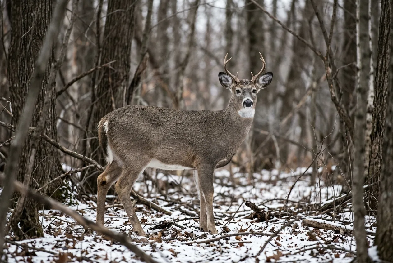
The single-vs-multiple-camera question. One finding that reliably surprises people: putting more cameras at each site can matter as much as adding sites. O'Connor and colleagues ran one-, two-, and four-camera setups at 20 forested sites and found the four-camera method detected 1.25 (53%) more species per site than a single camera, was the only configuration to fully detect the ground-dwelling community, and roughly doubled the number of sites where white-tailed deer were recorded. Detection probability for deer at a single camera was just 0.179. Their recommendation — "a minimum of 2 camera traps per camera-site, deployed towards opposite directions" — is a cheap hedge against the false negatives that wreck occupancy and richness data.
SECR density. The benchmark review found a median of 57.5 camera stations per study per year (mean ~100, range 12–849) across published SECR work. For jaguars specifically, Tobler and Powell concluded a minimum of 40–50 stations is required for a reliable survey, "and a larger number of stations would be desirable" — a threshold WildCAM repeats as the "bare minimum". SECR's saving grace is robustness: it's "much more robust to a smaller number of camera stations than other density estimation methods".
REM density. Simulation work suggests "c. 60 camera placements should be sampled to achieve acceptable precision (i.e. coefficient of variation below 0.20)".
To make the trade-offs concrete, here's how a few of the protocol-grade designs in the literature actually allocate cameras:
| Design / study | Stations & layout | Spacing | Density |
|---|---|---|---|
| TEAM tropical protocol | 60–90 points in 2–3 arrays of 20–30 | ~1.4 km | 1 camera / 2 km² |
| ForestGEO mammal protocol | 49–50 points, 7×7 or 10×5 grid | 140–145 m | 1 camera / 2 ha |
| Snow leopard "diffuse" | 44 cameras | ~5 km | 2 cameras / 100 km² |
| Snow leopard "compact" | 38 cameras | ~1 km | 15 cameras / 100 km² |
| Kays et al. recommendation | 40–60 sites per array | — | — |
Notice that ForestGEO deliberately runs cameras at a density 100-fold higher than TEAM — one trap per 2 ha versus one per 2 km² — because they're answering different questions over different areas (1 km² of intensive forest sampling versus 120 km² of community monitoring). Neither is "right." They're matched to their aims.
Coordinated and citizen-science surveys live at the far end of this spectrum: SNAPSHOT USA 2021, a multi-contributor national survey, pooled 109 camera trap arrays and 1,711 camera sites for 71,519 trap-nights, with effort per array ranging from 126 to 3,355 nights. The takeaway for anyone joining such a network is that consistency across contributors — standardized height, spacing, and duration — is what lets all those individually modest arrays be analyzed together at all.
ForestGEO deliberately runs cameras at a density 100-fold higher than TEAM, because they're answering different questions over different areas. Neither is "right." They're matched to their aims.
Why the extent of your grid can matter more than its density
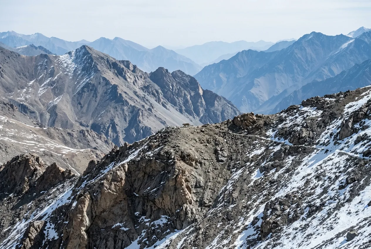
The snow leopard study is the cautionary tale every density surveyor should keep on the wall. The same team surveyed the same landscape two ways: a compact array (38 cameras, ~1 km spacing, 253 km² extent, 15 cameras/100 km²) and a diffuse one (44 cameras, ~5 km spacing, 2,030 km² extent — almost an order of magnitude larger — at just 2 cameras/100 km²).
The estimates didn't just differ — the compact design returned a density of 0.12 animals/100 km² against the diffuse design's 0.534, roughly five times higher in the diffuse layout. Worse, the compact array badly misrepresented how the cats actually used space, inflating the movement parameter σ̂ to 12.23 versus 3.27 in the diffuse design. The lesson the authors draw is the one Tobler and Powell drew for jaguars and the benchmark review drew across species: "sampling a small area approximately the size of a single home range is subject to biases resulting from very few individuals on the landscape with very low encounter probabilities". For density work, a grid that's tight and small can be far worse than one that's sparse and large. Cover enough area to expose enough individuals — that, more than packing cameras together, is what buys you a defensible estimate.
For density work, a grid that's tight and small can be far worse than one that's sparse and large.
Duration: how long to leave each camera, and how long to run the survey
Two different clocks are ticking, and people conflate them. One is how long a single camera should sit at one spot. The other is total survey length / total trap-nights. Both have good empirical anchors.
Per-camera duration. Kays et al.'s subsampling gives the cleanest guidance anyone has: running a camera for 2 weeks was most efficient for detecting new species, but 3–4 weeks were needed for precise local detection-rate estimates, "with no gains in precision observed after 1 month". Their headline recommendation — "run each camera for 3–5 weeks across 40–60 sites per array" — is now the de facto default for community studies. Si et al.'s intensive two-year study of a single Chinese plot adds a complementary rule: new species accumulate fast for the first ~40 days at a site, then the rate falls off a cliff, so they suggest rotating cameras "once c. 40 days" or after about 20 independent photographs.
Sites versus sessions — the recurring verdict. When cameras are limited (they always are), should you sample more sites for less time, or fewer sites for longer? For richness and relative abundance, the answer is consistent across studies: spread out. Si et al. found that, given the same total camera-days, "it was better to deploy cameras across more sites for a shorter time at each site, than to leave cameras at the same site" — at 1,000 camera-days, three sites detected 80% of species while 19 sites detected 90%. Kays et al. reach the same conclusion, and the WWF guide states it as policy: "sample more locations for a shorter period, rather than to sample just a few locations for a very long period". (Occupancy is the partial exception — for a rare, patchy species it's still better to move cameras and sample more sites, but for a common or a very poorly detectable species, sampling fewer sites for longer can actually be more efficient.)
Total trap-nights. Multiply the targets and you get a floor. The WWF guide's arithmetic — 20–50 locations × 30 trap-nights each — gives 600 to 1,500 trap-nights for a richness/diversity study, with a general recommendation that "diversity studies should be at least 1,000 trap nights". Si et al.'s rarefaction put the minimum at 931 camera-days to detect 90% of common species at their site, with about 8,700 camera-days needed to detect all 10 resident species — a stark illustration of how the long tail of rare species explodes effort. Burton's review found the median real-world effort was 2,055 trap-days, but flagged that nearly a third (28.9%) of studies had fewer than 1,000 total trap-days, "which is likely to be insufficient to detect rare species".
For density work the bar climbs. For relative abundance and REM, an index should rest on more than 10, ideally more than 20, captures — and "for densities typical of many carnivores (and the rarest ungulates), at least 2,000 trap nights will be required to obtain 20 captures". The SECR benchmark review found a median of 3,124 camera-days per year, with 71.6% of studies running a year or less. Jaguar surveys, because of the closure assumption, walk a tightrope: short enough to assume the population hasn't changed, long enough to gather data, with Tobler and Powell recommending a minimum of 60 days, often 90 or even 120 — explicitly rejecting the common 30-day window as too imprecise.
One sobering benchmark on whether all this effort actually pays off: across SECR studies, the median coefficient of variation was 30%, and "75.6% of studies reported a CV of ≤40%, but only 21% of studies reported a CV ≤20%". Most density surveys are not as precise as their authors would like. And only 10.5% of them ran any simulation before fieldwork to find out.
Most density surveys are not as precise as their authors would like. And only 10.5% of them ran any simulation before fieldwork to find out.
Detection probability is the hidden variable behind all of it
If there's one parameter that silently governs spacing, density, and duration, it's detection probability — the chance you photograph a species given it's there. Get it too low and your models don't just lose precision, they break.
The threshold to remember: detection probabilities below 0.2 "often lead to significant biases and convergence issues, even in the simplest single-state models". And the methods you might reach for to capture richer ecology make the problem worse — multistate occupancy models "require higher detection probabilities compared to the single-state models," and "the number of sites required was substantially higher for multistate models". The way detection and effort trade off is lawful: "minimum needed detection probabilities decreased as the number of surveys increased for all models". In other words, you can buy your way out of low detection with more survey occasions — to a point.
This is also why the seven-day occasion is so common: Kays et al. defined detection probability as "the probability of detecting an occurring species during a seven-day period at a camera site," aggregating daily data into weekly windows so that even sparsely-detected species produce workable detection histories. Pooling detections into multi-day occasions is a legitimate, no-cost lever for lifting detection probability and improving model fit. So is deploying more cameras per site. Both raise detection without the assumption-violations that bait and trail-targeting introduce — which brings us to the genuinely contested part of survey design.
Placement strategy and target species: the real fork in the road
Where you point the camera — on a game trail or at a random point — is the decision that splits the field, because it trades bias against data volume, and different species sit on different sides of that trade.
The evidence that placement biases your data is overwhelming and consistent. In Virginia, Kolowski and Forrester ran paired cameras and found detection probability rose 11–33% for five species on game trails versus random locations, and 24.9–38.2% for rodents at log features; in the most extreme case, a "mouse" category logged 65 capture events at logs compared to only a single capture at random locations. Capture rates ran 1.7 to 9.67 times higher at feature-based cameras. In Italy, Greco et al. deployed 60 cameras per strategy and recorded a mean of eight species on the trail network versus four off-trail, with wolf and wildcat yielding just five off-trail events each against 242 and 80 on trails — and 6-times more data overall on-trail. Eight of 11 species tested showed higher detection and occupancy on trails.
So trails win, right? Not for community work, and here's the bias they smuggle in: composition shifts. In the Italian study, wild ungulates made up 49% of relative abundance off-trail but only 28% on-trail, while carnivores flipped from 32% off-trail to 56% on-trail. You don't just get more data on trails — you get a differently shaped community, weighted toward the species that like trails. Cusack et al.'s paired savanna experiment in Tanzania pins down which: carnivores were significantly more likely to be caught at trail placements in the dry season, and larger-bodied species in the wet season. Their reassuring finding for richness surveys: "given adequate sampling effort (>1,400 camera trap nights), placement strategy is unlikely to affect inferences made at the community level" — but below that effort, and for specific trophic groups, it very much does.
This is where two authoritative sources point in opposite directions, and you need to understand why before you choose. For community, occupancy, and REM work, the guidance is emphatic that randomization is essential — non-random placement "violates a key principle of sampling theory: the random selection of sampling units," risks missing whole habitats and species, and biases relative abundance toward trail-users. But for SECR density of a marked, elusive species, Tobler and Powell recommend the reverse — place cameras "on well-established trails and logging roads that are frequently used by jaguars," because "cameras that are randomly placed in the landscape have a very low capture probability for jaguars and will result in poor data". The reconciliation isn't a compromise; it's the question again. If your estimator needs an unbiased sample of the community (random) versus enough recaptures of one cryptic individual to fit a spatial model (trail), the "right" placement genuinely differs — and if you mix trail and off-trail cameras, you record placement as a covariate so the model can account for it.
The deepest lesson is that species don't respond uniformly to any of this. Even similar-sized, closely-related species react differently to the same design choices, which is why some authors argue monitoring programs should employ a "mix of survey-design strategies" rather than one standardized approach when they care about a diverse community. (That paper's page was bot-blocked when its source file was captured, so this reflects the research pack's record of it rather than text I could read directly.) The practical move when you have one array and several target species: design for the hardest one — the rarest, lowest-detectability, widest-ranging species sets your spacing and effort, and the easier species come along for the ride.
You don't just get more data on trails — you get a differently shaped community, weighted toward the species that like trails.
Bait and lures: a tempting lever with a sting
Attractants raise detection, full stop. The question is what they cost you. In a 844-station test across Alberta, scent lure produced a strong positive effect on predators overall (β = 0.75) and a very strong effect on fisher (β = 2.23) — but no effect on gray wolf (β = -0.01, p = 0.973) and none on prey species or ungulates. That's the trap: lure helps some species, ignores others, and so "may introduce unknown bias into inferences across multiple species," meaning multispecies surveys "must account for the variable effect of scent lure".
The protocol-grade verdict reflects that. The WWF guide states plainly that "the use of attractants (baits and lures) is not recommended in formal camera trap surveys, unless there are very compelling reasons to use them and it is possible to control for their effects". TEAM uses no bait at all. The nuance from the occupancy-simulation side: bait and trail-targeting are widely used to push detection above that dangerous 0.2 floor, and the gain in model performance might be worth the bias — but data aggregation and multiple cameras per site achieve the same lift "without necessarily violating model assumptions," so reach for those first. If you do use bait, standardize it ruthlessly and record it as metadata so it can be modeled, not ignored.
The pitfalls that actually wreck datasets
Pulling the threads together, here's where camera trap survey design most often goes wrong — and every one of these is a design decision, not a field accident:
- No probability-based design. The 40.2% of studies placing cameras opportunistically can't generalize beyond the exact spots they sampled. Randomize, or stratify and randomize within strata.
- Too little effort for rare species. Under 1,000 trap-nights is likely insufficient to detect the rare species that matter most, and rare, low-occupancy species can need 100–150+ sites.
- A grid too small for the home range. For density, a camera polygon smaller than ~one home range carries a positive bias for every method tested.
- Treating one camera per site as enough. Single cameras miss detections that doubling to two opposing cameras would catch, distorting occupancy and richness.
- Ignoring seasonality. Kays et al. found 37–50% of species fluctuated significantly in occupancy or detection over the year, with temperate species varying in relative abundance by an average factor of 4–5 between seasons. A one-season snapshot is not the year. Pick your window deliberately and never compare across seasons without accounting for it.
- Confusing your "site." The same word covers a camera's detection zone and a 10-km² grid cell, and occupancy means different things at each scale. Define it.
- Not simulating first. Only ~10% of SECR studies ran a power analysis before fieldwork — the cheapest insurance against a precision-poor result there is.
Whatever you use, document the design itself as structured metadata — camera height and direction, spacing, duration, bait, detection-zone features — because a dataset whose design isn't recorded can't be reanalyzed or pooled with anyone else's. Standards like Camtrap DP exist precisely so survey design becomes part of the data, not lost institutional memory. If you want to go deeper on any one decision, the WWF best-practices guide remains the single most complete reference, and the Kays et al. paper is the empirical backbone for the "how many, how long" numbers.
Frequently asked questions
How far apart should camera traps be spaced?
It depends entirely on your goal. For richness, occupancy, or relative abundance you generally want independence, with a common rule of thumb of 1–2 km between stations (or at least one home-range diameter), though strict independence matters less than often claimed and can be handled statistically. For spatial capture–recapture density you want the opposite — cameras within about one-third of a home-range radius so individuals are caught at several stations, roughly 4–7 cameras per home range.
How many camera traps do I need for a survey?
For species richness, 25–35 sites cover most situations, with 50 a safer target. For occupancy, plan on 40+ for common species but 100–150+ for rare, low-occupancy species. For SECR density, 40–50 stations is a practical minimum, with a published median around 57 per study-year; REM simulations suggest about 60 placements for a coefficient of variation under 0.20.
How long should a camera trap survey run?
Run each camera 3–5 weeks — two weeks captures most new species, but precise detection rates need 3–4 weeks, with little gain past a month. For total effort, aim for at least 1,000 trap-nights for diversity work; many real surveys cluster around 2,000, and density studies of rare carnivores can need 2,000+ trap-nights just to log 20 captures.
Is it better to use more cameras or run them longer?
For richness and relative abundance, more sites for less time beats fewer sites for longer — at equal total camera-days, spreading cameras across more locations detects more species. The main exception is occupancy of a common or very hard-to-detect species, where concentrating effort at fewer sites can be more efficient.
Should I place cameras on trails or randomly?
For community, occupancy, and REM work, random placement is strongly preferred — trails bias your sample toward trail-using species and can shift the apparent community composition. For SECR density of an elusive marked species, targeting trails is often recommended to get enough recaptures, with placement recorded as a covariate.
Does using bait or scent lure improve a camera trap survey?
It raises detections for some species but not others — a strong effect on some predators, none on others or on prey — which introduces species-specific bias into multispecies surveys. Formal protocols generally advise against attractants unless you can control for their effects; raising detection through multi-day occasions or extra cameras per site is usually the safer lever.