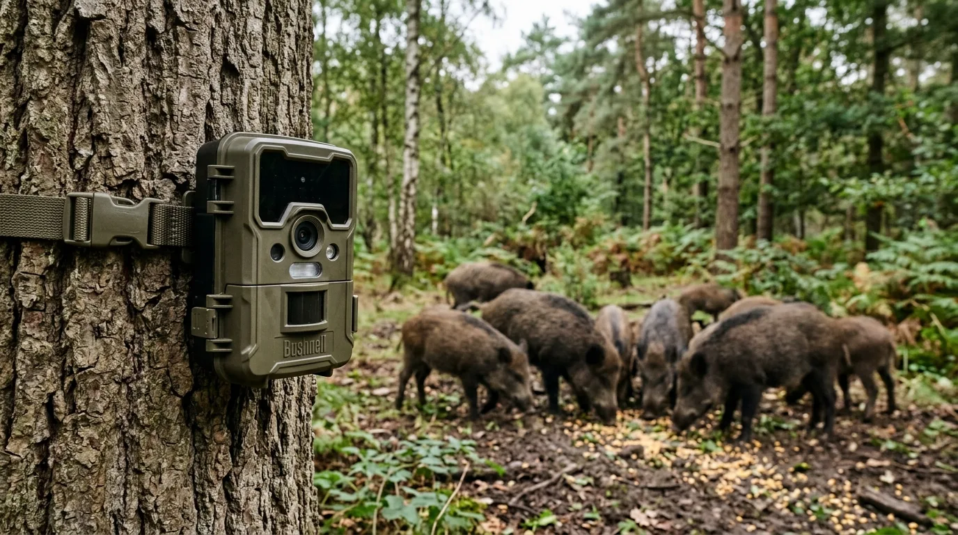
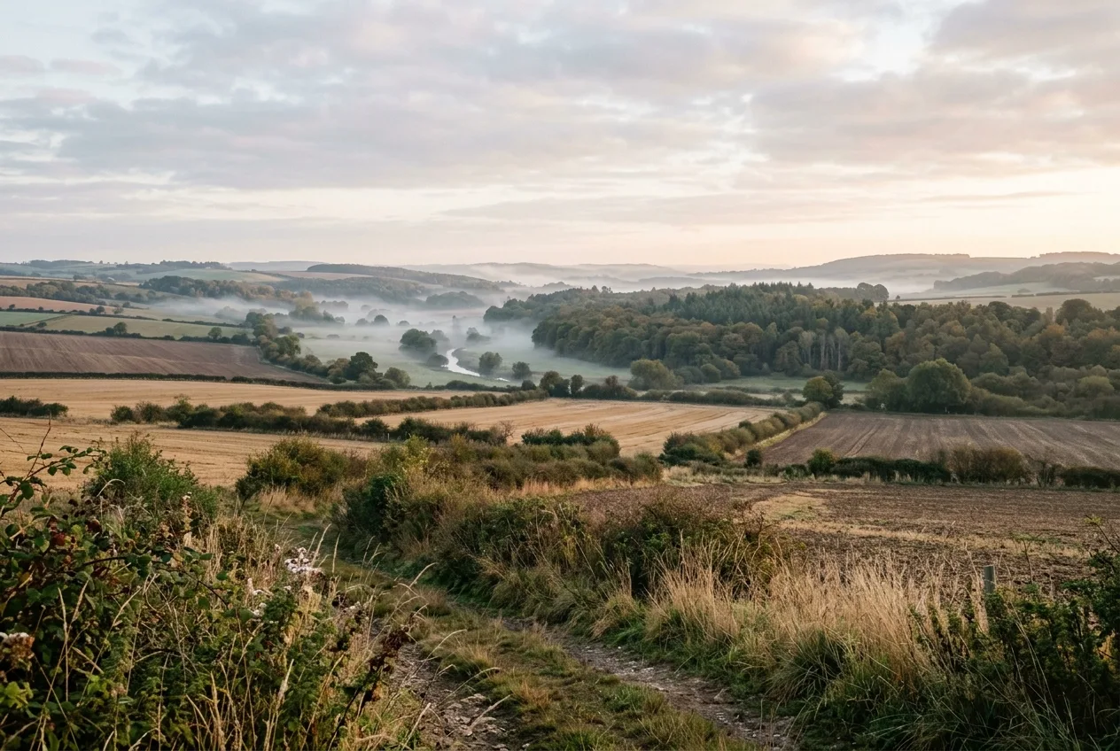
Here is the uncomfortable truth that shapes every wild boar count: the same bait that makes pigs show up for your cameras can wreck the math you were planning to run on them. Pour 50 pounds of corn in front of a camera and you'll get gorgeous, countable photos of sounders — and you'll also have pulled animals toward that spot from across their range, which quietly breaks the central assumption behind the most popular density models. So the first decision in any wild boar (or feral hog) camera survey isn't which camera to buy. It's deciding what you actually need: a number you can defend as a density, or a trend you can track over time. Those two goals point you at almost opposite field designs.
This guide walks through the real menu of methods practitioners use to turn trail-camera photos into wild boar population estimates — baited station counts, minimum-known-population, capture–mark–recapture and spatial mark-resight with ear-tagged sounders, the Random Encounter Model (REM) and its relatives (REST, space-to-event, time-to-event), N-mixture models, and camera-trap distance sampling. For each one, the question that matters most is the same: do its assumptions survive contact with how boar actually behave, and with the bait you put out? That's where good surveys are won and lost.
Why anyone counts boar in the first place
It helps to remember what these numbers are for, because it changes how precise you need to be. Wild boar and feral hogs are, in most of the places people survey them, a problem to be managed down rather than a population to be conserved. In the United States, federal agencies report that feral swine populations "have expanded across the country," with damage to agriculture estimated in the billions of dollars a year. Texas modeling makes the management arithmetic brutal in a way no camera can soften: with a current harvest rate around 29%, "up to 66% of the population will need to be removed annually for 5 years or more for the population to become stable". You cannot hit a removal target like that without some idea of the denominator.
You cannot remove your way out of a wild boar problem without knowing the denominator.
The disease angle has sharpened the need further. African swine fever (ASF) kills close to 90% of infected wild boar, and a population crash that severe ripples through the whole system — so agencies now want camera-based monitoring that can confirm a population has actually fallen, not just guess. And in Australia, where feral pigs are a long-standing agricultural pest, the management logic is stated plainly: monitoring before control should "establish a benchmark or index" of abundance so you have something to measure success against. Sometimes that's a true density; often a defensible index is all the decision needs.
The two honest framings: index vs. absolute density
Almost every method below sorts into one of two buckets, and conflating them is the single most common mistake.
An index of relative abundance is a number that goes up and down with the population but isn't itself a density — photos per camera-day, bait take, an occupancy estimate. Indices are cheap, robust, and perfectly adequate for "is this population bigger than last year, or smaller after we trapped?" The Australian agency manuals lean on indices for exactly this reason: complete counts of pigs "are rarely practical," so sample counts give "an index of abundance" instead.
An absolute density is animals per unit area — the thing you can multiply by your management area to get a population size. It's far more demanding, because now you have to account for the animals your cameras didn't see and the exact area each camera was watching.
An index tells you which way the population moved. A density tells you how many are there. Don't pay for one when you only need the other.
The rest of this guide is organized roughly from "index" toward "absolute density," because that's also roughly the order of increasing cost and assumption-load.
Baited camera-station counts: the workhorse index
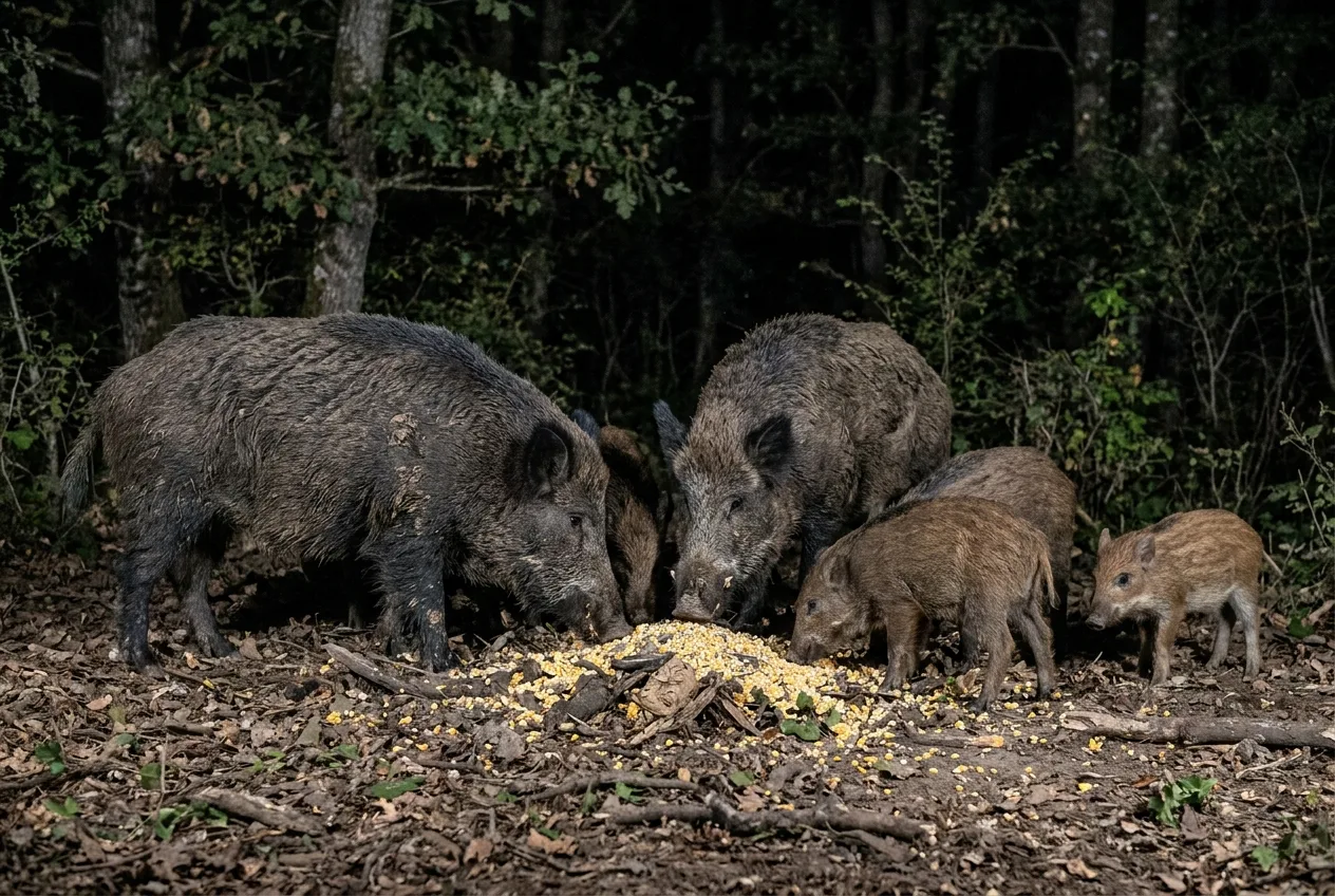
This is where most hog managers start, and it descends directly from the baited-camera deer survey Jacobson and colleagues popularized in 1997. The mental model is simple: bait a grid of camera stations, let pigs find them, then count what shows up — total pigs, distinct sounders, sex and age classes — over a short, fixed window.
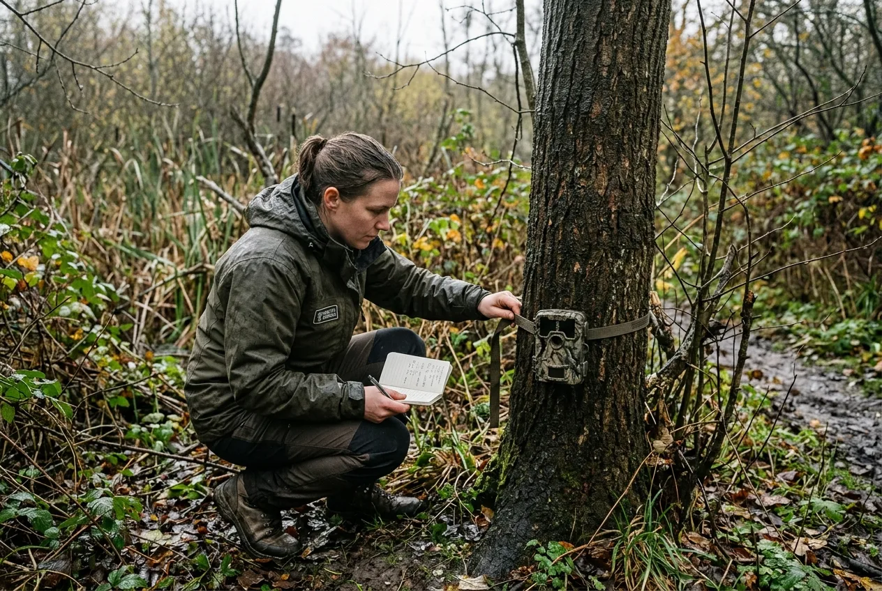
The "baited grid" has a fairly settled recipe in the hog literature. A USDA wild-pig study ran a 5×4 grid of 20 cameras spaced 750 m apart (±75 m), baited each station with 22 kg of whole corn on the ground in front of the camera, set a 3-minute trigger delay, and ran it for 12 days. The Rapid Population Assessment (RPA) protocol developed across Florida, California and South Carolina sites is built on the same bones: baited camera grids spaced roughly 500 or 750 m apart, with each grid deployed twice, a few months apart, to catch seasonal or post-control change.
Two practical findings make these surveys efficient. First, you don't need to run them long. Monitoring 73 pre-baited feral-pig stations through seven straight 24-hour periods, detection probability for every class — adult sows, adult boars, juveniles — exceeded 0.5 by the third day. The authors' recommendation: hold sampling to "three 24-hour periods per monitoring station following a uniform pre-baiting schedule," which cuts cost, limits human scent at the bait, and avoids the perverse effect of prolonged baiting actually boosting pig survival and productivity. Second, most boar movement is nocturnal, so for adults you can largely sample at night with little loss — though juveniles get missed slightly more often after dark.
What do you get? Not a density on its own — but the RPA work showed something useful: occupancy, detection probability, and N-mixture estimates from those baited grids were all "positively correlated with spatially explicit capture-recapture density estimates". In other words, the cheap baited-grid indices track the expensive density estimate well enough to monitor trends and judge whether control worked. And the obvious design lever holds: adding cameras increases precision.
The Canadian OFAH protocol is worth flagging here precisely because it's honest about its own limits. It's a detailed, well-built citizen-science scheme — trigger speed ≤0.5 s, ≤1 s between photos, 3–5 photo bursts, camera ~1 m up a post facing the bait, faced toward the pole (north up north, south below the equator) to dodge sun-triggered false fires, with a walk-test before you leave. But it states flatly that it "is not intended to avoid bias in any way and prioritizes only wild pig detection rather than abundance or occupancy information". That's the right disclaimer. A baited camera tells you pigs are there; turning "there" into "how many" takes more.
A note on bait itself
Bait choice is a survey-design decision, not an afterthought. Corn is the standard hog attractant, but straight whole corn is discouraged in winter because it can be toxic to non-target deer — mix it at least 1:1 with whole oats, or use soured (fermented) corn, which deer find less attractive. Spread bait across the site rather than dumping it in a pile. And remember the lesson buried in all of this: the bait that's helping you here is the same bait that will sabotage a REM density estimate later.
Minimum-known-population and capture–mark–recapture
If a baited camera survey runs long enough and you can tell individuals apart, you can at least state a minimum known population — the count of distinct animals you positively identified. In the Fort Benning detectability study, researchers identified 348 unique feral pigs from over 240,000 images by sex, approximate weight, pelage and group association, with some animals carrying ear tags from earlier work. That distinct-individual count is a hard floor: at least this many pigs used the area. It's a useful sanity check, but it's a minimum, not an estimate — it says nothing about the animals you never photographed.
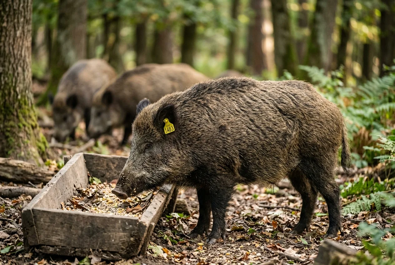
Capture–mark–recapture (CMR) turns marking into a real estimate. The logic is the classic one: mark a sample of animals, then see what fraction of later detections are marked; the smaller that fraction, the larger the population. Feral pigs cooperate with this better than most wildlife because they're relatively trappable. As the NSW manual puts it, "because feral pigs are relatively trappable, capture–recapture studies can work well for these animals" — trap them, ear-tag and release, then use recapture rates to estimate the number in the sampled area. The cameras come in as the resight leg: rather than physically recapturing every pig, you let cameras photograph the marked and unmarked animals, which is far less invasive.
The catch is that wild boar are only partly markable. They have no natural individual markings, so you have to physically catch and tag a sample — which means ethics approval, trained staff, and real cost, and it gives up the non-invasive appeal of cameras. That fundamental fact pushes the field in two directions: toward methods that need only a few marked animals (spatial mark-resight), and toward methods that need none (the unmarked models).
Spatial mark-resight and SECR: density from marked sounders
Spatially explicit capture–recapture (SECR) is the gold standard for marked species, and it's what gives you density rather than a population-of-unknown-area. Instead of just counting marks, SECR uses where each detection happened to estimate each animal's activity center and how detection falls off with distance — which means the area is built into the estimate, not guessed afterward.
But SECR was built for, and works best on, animals that are "large-ranging, rare and elusive, and individually identifiable" — think spotted and striped cats, where every individual is a walking barcode. Boar aren't that. The workaround is spatial mark-resight (SMR), an extension of SECR for partially marked populations. A Spanish study did exactly this for wild boar: they captured and ear-tagged seven boar (two also wearing GPS collars), deployed 61 cameras at 500 m spacing, and analyzed marked and unmarked animals together with a generalized SMR model designed to handle the reality that you can't always read a tag in a night photo.
A second route to a marked population skips ear tags entirely and reads DNA from feces. In a head-to-head on the same South Carolina wild-pig population, a fecal-DNA mark-recapture estimate, a camera-SECR estimate, and a removal estimate all landed at similar densities. That agreement is reassuring — but the costs were not equal, which brings us to the most useful single comparison in this literature.
Three different methods, run on the same pigs, gave the same density — at three very different prices.
In that study, camera sampling was the least expensive at roughly \$10,500, removal sampling came in around \$15,000, and fecal-DNA was the priciest at about \$17,700 (71% of it labor, much of that lab work). The camera method's weakness was precision: it "was the least expensive, but had large variances". And about half the camera labor went to a step that has nothing to do with the field — roughly 51% of the camera effort was spent examining and classifying the images. The authors' honest bottom line is one every survey designer should internalize: there is no universally best method, and "the preferred method … will therefore be dependent on the unique conditions of that study system".
The unmarked models: density without individual ID
This is the most active corner of the field, and the reason cameras are now a credible density tool for boar at all. These methods — sometimes called viewshed density estimators — translate raw detection rates into density without ever identifying an individual. They're attractive because they drop the need to capture, tag, or even distinguish animals. They're dangerous because each one rests on assumptions that boar behavior and baiting can quietly violate.
The Random Encounter Model (REM)
REM is the foundational one, and the mental model is genuinely elegant: treat animals like gas molecules bouncing around a space, and cameras like fixed detectors they randomly bump into. If you know how often animals hit the detector (the encounter rate), how fast they move (their daily travel distance, or "day range"), and the size of the camera's detection zone (its radius and angle), you can back out density. Crucially, REM needs no individual recognition, and because its design isn't tied to recapturing the same animal twice, one survey can estimate density for several species at once.
REM's reliability now has solid backing. Tested against independent reference methods across 13 populations of ungulates and a lagomorph — wild boar included — REM came out "a reliable method for estimating wildlife population density when using appropriate estimates of REM parameters and sampling designs". Applied in an ASF-hit Italian park, REM put post-outbreak wild boar at 0.27 individuals/km² (±0.11) and, in the same survey, harvested the very parameters it needs from the camera data: a day range of 9.07 km/day and an activity level of 0.49, meaning the boar were active about 11.76 hours a day.
But REM is unforgiving about its inputs, and this is where boar surveys go wrong. The Spanish review is blunt about the failure modes: "deficient estimates of day range and encounter rate lead to an overestimation of density, while deficient estimates of detection zone conducted to underestimations". Get the movement speed wrong and you overshoot; mis-measure the detection zone and you undershoot.
And then there's the assumption that should be tattooed on every REM practitioner's arm. REM assumes "cameras are placed randomly with respect to animal movement," meaning they "should not be targeted so as to inflate, or deflate, encounter rates". Bait does exactly the forbidden thing. When a Serengeti lion study placed cameras at shady trees the cats favored, every REM model over-estimated density — and the fix was to restrict the data to periods when the animals' movement was closer to random, which alone brought estimates in line with the truth. The lesson transfers directly: a baited wild boar camera is the savanna shade-tree all over again. If you want REM density, your cameras go on a systematic or random grid, unbaited.
REST, space-to-event and time-to-event
REM's biggest practical headache is that you need an animal's day range, which often means telemetry. The newer estimators chip away at that.
REST (Random Encounter and Staying Time) replaces movement speed with staying time — how long an animal lingers in a small, defined zone in front of the camera, which you measure straight off the video. A Japanese team used REST inside a Bayesian model that also estimated trap catchability, deploying 180 cameras over 800 km², and tracked boar density rising after the spring birth pulse and falling through winter harvest. (A nice management byproduct: they found box-trap catchability ran about 1.7× snare-trap catchability and that both peaked in winter, when hungry boar range farther — so trapping effort pays off most in the cold months.)
Space-to-event (STE) and time-to-event (TTE), along with instantaneous sampling, go further and "treat remote camera data like point counts". TTE uses the time until the first detection; STE uses how much sampled space you have to search before the first detection. The headline advantage for a fast, lingering animal like a boar: in testing, all three "produced unbiased estimates of abundance, regardless of animal movement rate" — so STE in particular sidesteps the day-range problem that dogs REM.
Camera-trap distance sampling (CTDS)
CTDS borrows the well-worn distance-sampling framework — the one wildlife agencies have used from transects for decades — and points it at cameras. You measure the distance from the camera to each animal in the frame, fit a curve describing how detection drops off with distance, and account for the fraction of time animals are even available to be seen (boar resting out of view don't count). It's the method behind one of the cleaner European boar density figures: in Portugal's Peneda-Gerês park, a 64-camera grid over 16 km² produced a 2019 wild boar density of 2.59 individuals/km² via CTDS.
N-mixture models
N-mixture models estimate abundance from repeated counts while correcting for imperfect detection, and they have one big draw: they need no extra fieldwork beyond the counts themselves. The trade-off is that they don't explicitly estimate the area sampled, so they're best read as relative abundance rather than true density. Run against REM on the same Spanish boar population over five winters, N-mixture and REM agreed to the same order of magnitude — REM put boar at 5.34–7.14/km² — and the practical guidance is refreshingly clear: "when all that is needed are relative population trends, applying NMM may be faster, cheaper". The caveat: that agreement holds "when the range of variability is large," but the two methods can disagree on finer year-to-year wobbles.
Comparing the methods at a glance
| Method | What it needs in the field | Key assumption (where it fails for boar) | What you get | Baiting OK? |
|---|---|---|---|---|
| Baited station / RPA grid | Grid of baited cameras, short run (3–10 days) | None for an index; but counts aren't density | Relative abundance index; tracks change & control | Yes — that's the point |
| Minimum known population | Long enough survey to ID distinct individuals | Assumes you saw a meaningful share | A hard floor, not an estimate | Yes |
| CMR / spatial mark-resight (SMR) | Trap & ear-tag a sample; cameras resight | Boar only partly markable; tagging is invasive | Population size (CMR) or density (SMR) | Baiting traps is normal; resight design matters |
| Camera SECR | Marked/identifiable individuals across the array | Built for identifiable cats; boar aren't | Density | Generally unbaited array |
| REM | Encounter rate, day range, detection zone | Random camera placement; bait breaks it | Absolute density, multi-species | No |
| REST | Encounter rate, staying time, detection zone | Correct staying-time & active-time measurement | Absolute density | No |
| STE / TTE | Detection events + sampled area; point-count style | Correct sampled-area; random placement | Abundance, movement-insensitive | No |
| CTDS | Distance to each animal; availability fraction | Correct distances & detection function | Absolute density | No |
| N-mixture | Repeated counts only | Doesn't model sampled area → relative, not absolute | Relative abundance / trends | Index use is fine |
| Occupancy | Detection/non-detection across sites | Grid often smaller than boar range → "habitat use," not occupancy | Change/trend signal | Either |
Spacing, effort and duration: the design dials
A few numbers recur across the boar and camera-density literature and are worth holding onto.
Spacing. For SECR-type work, the rule is to put "more than one trap within the average home range size of the species" so the same animals get detected at multiple cameras. The hog grids cluster tighter than that: 750 m in the USDA wild-pig study, 500–750 m for the RPA grids, roughly 500 m in the Portuguese CTDS grid (one camera per quarter-hectare cell), and 500 m for the SMR boar array. For unmarked REM-type surveys, camera spacing isn't dictated by the target species at all, which is part of what lets one survey serve several species.
How many cameras. Because real boar populations are spatially clumped, precision is hard-won. A REM simulation suggested "c. 60 camera placements should be sampled to achieve acceptable precision" — a coefficient of variation below 0.20. That's a sobering bar: across 95 SECR studies reviewed, only 21% actually hit a CV of 20% or better, meaning most camera surveys are underpowered. The practical move is to run a power analysis before fieldwork — tools like the `secrdesign` package exist precisely so you can size the array to your target precision rather than discovering it was too small afterward.
Duration. For baited hog grids, short is better: three 24-hour periods after pre-baiting clears the detection bar for all classes; the USDA grid ran 12 days; and the RPA grids were each deployed twice, a few months apart, to catch change. For removal-based estimates, the opposite — more traps and "14 or more days" of trapping yield the least biased numbers. And for genuine trend detection, you commit to years: the boar trend comparisons spanned five consecutive winters.
Double-counting and detection bias: where the numbers quietly lie
Two failure modes deserve their own section because they sink otherwise-careful surveys.
Double-counting. A boar that strolls through a camera's view, stops to root, and triggers forty photos is one animal, not forty events. The standard discipline is to define an "independent" detection as the animal entering and exiting the field of view, and to treat consecutive frames of a stationary animal as the same event. Group-living complicates it further: a sounder is several pigs arriving together, and how you handle group counts feeds straight into density. Get the event definition sloppy and your encounter rate — and your density — inflates.
Detection-zone error. This is the silent killer of camera densities. Every viewshed estimator "is sensitive to measurements of the sampled area in front of cameras," and a proportional error in that area becomes a proportional error in density. The fix is to measure the detection zone in the field rather than trusting the spec sheet — and the gap between the two is real: in the Portuguese survey, many cameras only detected animals out to about 10 m even though the sensor was rated to 30 m. The geometry matters too. Standard REM assumes a horizontal camera with a wedge-shaped detection zone; if you mount cameras pointing straight down (a trick to foil theft), the effective area becomes a rectangle and the formula has to change accordingly. Either way, getting the zone wrong skews density — typically downward when you overstate the area, upward when you understate it.
There's also detection bias you can't see in a single frame: if your detection probability isn't constant — say juveniles are harder to catch at night, or pigs are warier near roads — naive counts drift. Occupancy and N-mixture models exist largely to model that imperfect detection explicitly. One honest caveat from the occupancy literature on boar: when your camera grid cells are smaller than a boar's home range, "occupancy should be interpreted as habitat use" rather than true occupancy. The model still tracks change usefully — Belgian researchers used it to confirm an ASF-driven crash, with boar occupancy at 0.235 in infected zones versus 0.868 in clean ones — but you have to call it what it is.
The fastest way to a confidently wrong boar density is a detection zone you assumed instead of measured.
If there's a place where the trail.cam workflow earns its keep in a survey like this, it's the unglamorous middle: half the labor in the South Carolina camera study went to a human sorting and classifying images, and a single European boar grid generated nearly a million photos.
How agencies actually do it, by region
The method you reach for is partly a regional habit, shaped by terrain and policy.
In Europe, the EFSA-funded ENETWILD network reviewed eighteen methods and recommended three for estimating wild boar density at a local (management-unit) scale: camera trapping, drive counts, and distance sampling with thermography; for large-scale, long-term trends across the continent, it judged high-quality hunting-bag statistics the most practical and comparable option. Camera-based REM and CTDS show up repeatedly in the European boar studies for the local, defensible-density end of that spectrum.
In the United States, the federal program frames method choice around "the landscape and environmental conditions, feral swine behavior and density, as well as local regulations", and the USDA-authored studies lean on baited camera grids, camera-SECR and removal models for the density work. In Australia, the agency tradition is a menu of indices — index-removal-index, bait-take, dung counts, spotlight counts, CMR — with cameras adopted later for monitoring; the National Feral Pig Action Plan documents landscape-scale camera monitoring and even real-time alert cameras that notify landholders of pig activity. And Canada's OFAH protocol is unapologetically a detection tool — designed to find newly arrived pigs early, not to count them.
If you want one case study that ties the whole loop together, it's the Western Riverina in New South Wales: an annual aerial survey with infrared cameras set the baseline density, control ran for years, and the program documented density falling "from 11.6 pigs/km² at the start of the program to 0.6 pigs/km² at its conclusion". That's the payoff of getting the count right — you can prove the management worked.
Frequently asked questions
Can I get a real wild boar density from baited trail cameras?
Not a clean absolute density. Baiting concentrates pigs and makes camera placement non-random, which violates the core assumption of REM-type density models and inflates encounter rates. Baited grids are excellent for a relative-abundance index that tracks change — and those indices correlate well with proper density estimates — but for true density you want unbaited, systematically or randomly placed cameras.
How many cameras and how long do I need?
For a baited index survey, short and dense works: three 24-hour periods per station after pre-baiting clears the detection bar for all age classes, and grids of ~20 cameras run 10–12 days are typical. For absolute density, simulation suggests around 60 camera placements to reach good precision, because boar cluster spatially — and most past surveys were underpowered, so run a power analysis first.
Why can't I just use SECR like people do for big cats?
SECR needs individually identifiable animals, and it shines on "large-ranging, rare and elusive, and individually identifiable" species like spotted cats. Wild boar have no natural individual markings, so you'd have to ear-tag a sample and use spatial mark-resight instead, read individual identity from fecal DNA, or switch to an unmarked model that needs no individual ID at all.
Which method is cheapest?
On a like-for-like wild-pig comparison, camera sampling was the least expensive (~\$10,500) versus removal (~\$15,000) and fecal-DNA (~\$17,700) — but the camera estimate had the largest variances, and about half its cost was the labor of classifying images, not fieldwork. Cheapest isn't free of trade-offs.
Does it matter how I mount and measure the camera?
A great deal. Every camera density model is sensitive to the area each camera samples, and field detection zones are often far smaller than the spec sheet claims — frequently ~10 m versus a rated 30 m. Measure the detection zone in the field; if you mount cameras vertically to prevent theft, the detection area becomes a rectangle and the math changes.
What's the difference between REM and REST?
Both estimate density without identifying individuals. REM needs the animal's daily travel distance (day range), which usually means telemetry or careful camera-based movement analysis. REST swaps that for "staying time" — how long an animal lingers in a defined zone, measured directly from the video — which removes the hardest parameter to get.