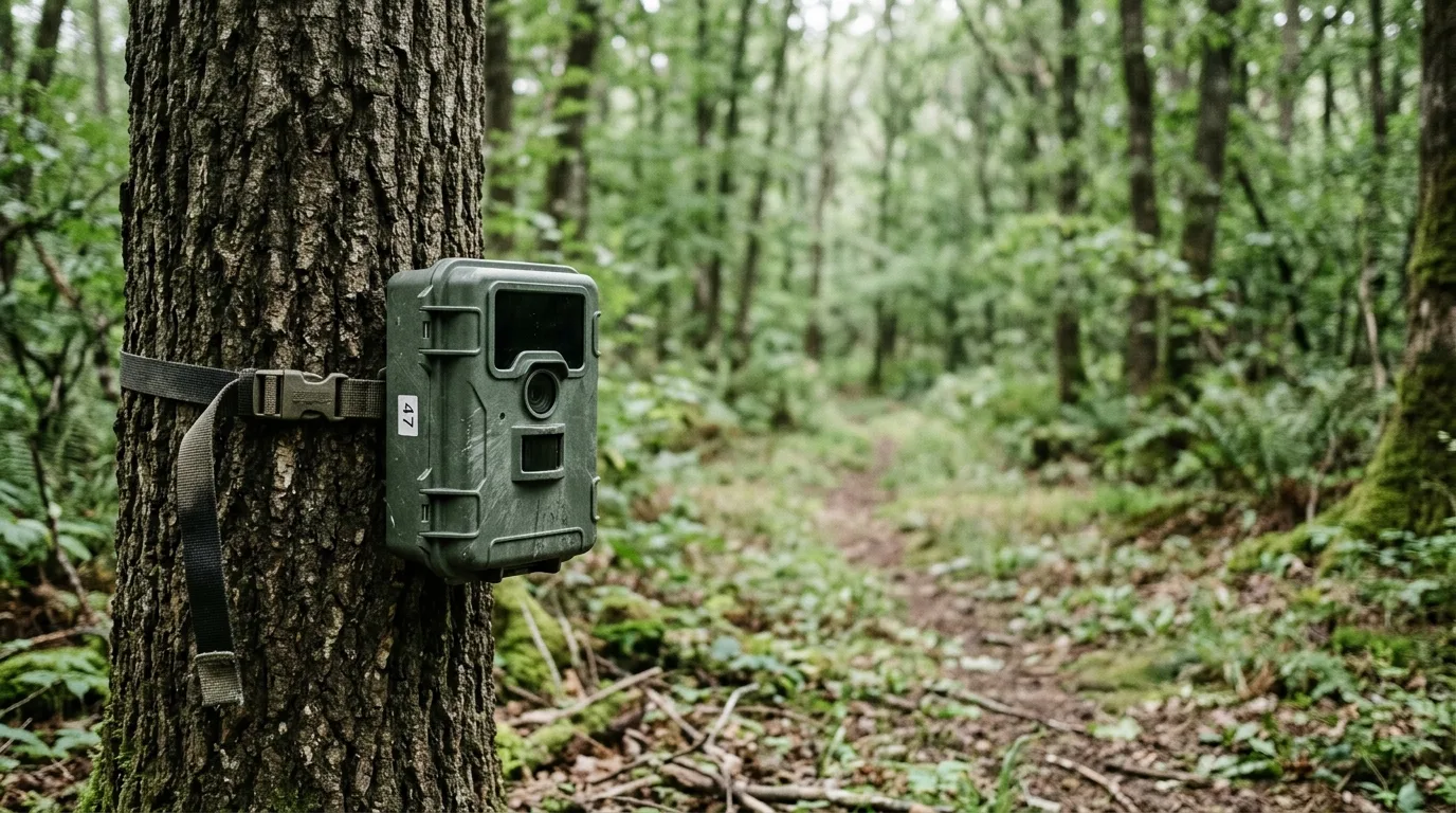
A camera that fires a thousand times tells you almost nothing about how many animals live in front of it. It could be a thousand different deer passing once, or one bold fox that learned the lens makes a satisfying chew toy. That ambiguity — many mobile individuals versus one busy resident — is the whole problem. It's why a raw "trap rate" has never been a trustworthy currency, and why, for decades, camera-trap density estimation meant tigers, leopards, and not much else: you needed individually recognizable coats to run capture-recapture.
Most species don't have stripes. A red fox is a red fox. So a family of methods grew up to do something that sounds almost too clever — estimate absolute density, animals per square kilometre, from unmarked animals you can't tell apart. This is the guide to that family: the Random Encounter Model and its descendants, what each one actually needs from you, and the specific ways each one will lie to you if you're not careful. None of them is magic, and — this matters — none of them is the universal answer. The honest state of the field is a set of trade-offs, not a winner.
If you've read our pieces on Camera Trap Survey Design: Spacing, Density, and Duration or How to Count Wild Boar with Trail Cameras: Baited Surveys and Population Estimates, this is the analytical layer that sits underneath: you've placed the cameras, you have the detections, now you want a number with units on it.
Why "just count the photos" was never going to work
Two things break the naive approach. First, the individual-identity problem already mentioned: detections don't map cleanly to animals. Second, and more subtly, animal movement smears the sampling area. A camera samples some patch of ground, but how big is that patch? It depends on how far the animals you're trying to count typically roam, which you usually don't know. Without a defined sampling area, an abundance estimate has no denominator — no clear space it refers to.
So the field splits, really, on how each method handles that space problem. Some estimate abundance at a camera with no spatial reference at all and make you assign it to an area afterward. Some build the area explicitly into the model. And some — the ones this guide leans on — estimate density directly within the cameras' collective field of view and assume that view represents the wider landscape. That last assumption, "the cameras see a fair sample," is doing enormous work, and it's exactly why placement discipline turns out to matter more than any modelling choice.
Here's a number that should reframe how you think about this whole enterprise. A review of 927 camera-trap studies published between 2014 and 2019 found that only about 5.5% used any abundance-estimation method at all. The overwhelming majority fell back on relative-abundance indices, occupancy, or behaviour. The methods below are not the well-trodden default. They're a frontier, and they reward people who understand their assumptions rather than treating them as a black box.
A camera that fires a thousand times tells you almost nothing about how many animals live in front of it.
The Random Encounter Model: animals as gas particles
REM is the founder, and its central idea is borrowed, beautifully, from nineteenth-century physics. Physicists modelled how often gas molecules collide. Rowcliffe and colleagues realized that animals bumping into a camera's detection zone is the same kind of process. Treat animals like ideal-gas particles moving randomly through space, and the rate at which they trigger a camera becomes a predictable function of how many there are, how fast they move, and how big the detection zone is.
In practice that means REM scales trap rate to density using four ingredients: average group size and day range (how far an animal travels in a day) on the biology side, and the radius and angle of the camera's detection zone on the hardware side. Get unbiased estimates of those, place your cameras without bias, and the photos give you density.
The original field test is instructive precisely because of where it failed. In an enclosed English wildlife park with known animal numbers, REM nailed three of four species to within 22% of the true count. The fourth — a small marsupial called the mara — came out 86% too low. The reason wasn't the model. It was that roughly 90% of the mara grazed on open lawns where the researchers had deliberately not placed cameras, to avoid photographing visitors. The lesson has echoed through every paper since: the moment you let camera placement correlate with where animals are, REM breaks. No targeting trails, sign, water holes, or bait to juice your capture rate — that violates the observation model and "cannot give unbiased density estimates".
The second recurring headache is day range. Knowing how far your study animals travel per day, without bias, is genuinely hard. Allometric shortcuts (estimating day range from body size) "introduce large bias and should be used cautiously". You can get it from GPS collars, but a black-bear study made the failure mode vivid: collar fixes taken at long intervals underestimate how far an animal actually moved, which in turn overestimates density — and the bias bites harder for slow-moving species. In that same study, REM landed a credible black-bear density that wasn't significantly different from a DNA-based spatial capture-recapture reference, but only once the speed input was handled with care. The catch is almost philosophical: if you need expensive collar data to feed REM, you've lost the cheap-and-noninvasive advantage that made REM attractive in the first place.
Apply REM to a species that doesn't behave like a gas particle and you can see the strain directly. Female lions in the Serengeti spend their days dozing under isolated trees — and isolated trees are exactly where you'd put a camera. Every REM model in that study overestimated lion density; restricting the analysis to night-time photos, when lions actually move, cut the bias substantially. That's the recurring REM craft: find the times and places where your animals move randomly with respect to the cameras, and lean on those.
The moment you let camera placement correlate with where animals are, the Random Encounter Model breaks.
Distance sampling for cameras (CT-DS): borrow a 50-year-old toolbox
Camera-trap distance sampling makes a different bet. Distance sampling — measuring how detection falls off with distance from an observer — is one of the most mature, best-supported frameworks in all of wildlife survey, with decades of theory, software, and design guidance behind it. Howe, Buckland, and colleagues adapted point-transect distance sampling so that a camera plays the role of the observer.
The mechanic is elegant. Instead of trying to estimate animal speed, CT-DS records the radial distance to each animal at predetermined snapshot moments a couple of seconds apart, and models how detection declines with distance. Because the snapshots are fixed clock times chosen independently of where animals happen to be, movement doesn't bias the distance distribution. You inherit the entire distance-sampling apparatus — program Distance, model-selection conventions, the lot — and you never have to estimate day range.
What CT-DS demands in return is certain detection right in front of the camera (distance zero). Small animals slipping under the field of view, half-bodies that can't be identified, or a sluggish trigger all violate it — and the fix is to left-truncate, discarding the near-camera distances where detection isn't certain. It also can only count animals that are available to be seen: a species that spends half its time underground or in the canopy reads as half its true density unless you correct for that unavailable time.
CT-DS shines at scale and across many species at once. In a survey of Salonga National Park in the Democratic Republic of Congo — 160 cameras spread over 17,000 square kilometres — a single CT-DS deployment produced density estimates for 14 species simultaneously, from a 200-gram elephant shrew to forest elephants, including the first-ever density figures for the Congo peafowl and the giant ground pangolin. That multi-species reach is something REST and TIFC struggle to match.
But Salonga also exposed CT-DS's nastiest failure mode: animals reacting to the camera. Forest elephants found the cameras fascinating and lingered in front of them, smelling and investigating. Including those reactive observations inflated elephant density by up to two orders of magnitude. Bonobos did the opposite — hanging back warily — which inflated their density by about 15%. The recommended defences are to deploy cameras a month ahead so animals habituate, or to favour a method less sensitive to reactivity for the worst offenders.
There's also a quieter CT-DS trap worth knowing about, because it's easy to miss and the consequences are large. CT-DS was designed for video. If you run it on still images, the camera goes blind during its recovery time and during periods when a stationary animal fails to re-trigger it. Fail to subtract those dead intervals from your survey effort and you can underestimate density by up to 96% — because you've credited the camera with sampling time it spent asleep. The mean dead interval in one European study ran 8 to 15 seconds depending on species, which adds up fast.
REST: trade speed for staying time
The Random Encounter and Staying Time model is REM's clever Japanese cousin. It keeps REM's encounter logic but swaps out the parameter everyone hates — day range — for one you can read straight off the footage: staying time, how long an animal lingers in a small, predefined focal zone where you're confident detection is certain. Because staying time is inversely proportional to speed, it carries the same information without you ever having to collar anything.
REST has a property worth pausing on: in simulations it stayed unbiased even when individual animals moved at different speeds, and even when they travelled in pairs. That robustness is real and valuable. But REST comes with a famously explicit rap sheet — the authors list seven assumptions outright. Two of them cause most of the trouble in the field. First, if animals are not active in synchrony — some asleep while others forage — REST underestimates density. Second, an animal that flops down and rests inside the focal zone produces a freakishly long staying time that drags the mean up and overestimates density; the fix is to discard those outliers and correct your effort by the fraction of the day animals are actually active.
The practical setup is fussier than REM's. You define a focal area — an equilateral triangle works best — usually around 1.9 metres on a side, centred in the field of view, and you verify that detection inside it really is certain. You run the camera with no delay between triggers (a delay inflates your effort calculation and biases density down), with fast sensors and generous battery, ideally recording video longer than 15 seconds. Then comes the labour: superimposing a reference image of the empty focal zone over each animal clip to measure exactly how long it was inside. The authors of the practitioner's guide are refreshingly blunt that this measurement is "labour-intensive and in its infancy".
The payoff, in the one head-to-head trial that tested all the major methods together, was the best precision and the lowest human effort of the three. The catch is the flip side of that efficiency: because REST only uses animals that cross the small focal triangle, it runs short of data for low-density species — the very situations where you most want a number.
TIFC: the camera as a quadrat
Time-in-front-of-camera takes the staying-time idea to its logical extreme and arguably makes it the most practitioner-friendly of the lot. Forget separating encounters from staying times. Just add up the total time any animal of your target species spent in the field of view over the whole deployment, divide by the area sampled and the total operating time, and you have density.
The reason this works is genuinely satisfying. Cumulative time in view is invariant to how fast animals move and how big their home ranges are. Double an animal's speed and it spends half as long in frame on each pass — but it passes twice as often. Double the home-range size and it visits any given camera half as often — but there are twice as many animals whose ranges overlap that camera. The bookkeeping cancels, leaving you with a measure that needs no movement rate, no group size, and no home-range input at all. For that reason it has been deployed at enormous scale: nearly 3,000 cameras across Alberta over six years.
TIFC's assumptions are the same family as the rest — representative placement, no camera-induced behaviour change, reliable detection near the camera — but its signature weakness is the one staying-time methods all share, and TIFC feels it acutely because it counts every second: animals that linger inflate the estimate. A recent ungulate study spelled out exactly how this plays out across species, and it's the clearest cautionary tale in the literature. Compared against aerial surveys, TIFC nailed moose (solitary, doesn't loiter). It came out 19% low for bison, because the cameras under-sampled the open grasslands bison favour. And it ran a startling 116% high for elk, because the cameras sat on game trails (where elk concentrate) and elk kept stopping to investigate the lens — both inflating staying time. Correction factors helped, but the authors warn those factors may need re-tuning for each landscape. The takeaway isn't "TIFC is bad." It's that the same method can be unbiased, biased low, and biased high for three species in the same dataset, entirely because of placement and behaviour.
The same method was unbiased for moose, biased low for bison, and biased high for elk — in one dataset, entirely because of where the cameras sat and how the animals behaved.
Time-to-event and space-to-event: counting the clock and the gaps
The newest branch came from biologists thinking like survival analysts. If a camera records events continuously, then the time until the first animal shows up carries information about abundance. That's the time-to-event (TTE) model. The problem is that TTE, like REM, depends on an independent movement estimate and is therefore sensitive to movement speed — in simulations it tended to underestimate, badly so for slow-moving populations.
So the same team did something neat: they collapsed each sampling occasion to a single instant. If you only look at one frozen moment, animal movement during the interval can't bias you. That's the space-to-event (STE) model, and its estimates are insensitive to movement rate entirely. STE uses time-lapse photos — frames taken on a schedule rather than by motion trigger — which carries a second, underrated advantage: it sidesteps the whole problem of variable motion-sensor detection, because a scheduled frame either contains an animal or it doesn't. A further simplification, instantaneous sampling (IS), just counts animals in each time-lapse frame as a fixed-area sample.
In a field test on wintering elk, STE delivered the best precision of the new methods without needing any movement input, landing close to an aerial survey's tally. These methods also quietly solve labour problems: TTE lets a reviewer stop scanning images after the first detection, and STE lets you estimate abundance without counting how many animals are in each photo — a real saving, since per-photo counts are slow and error-prone. The trade-off is that time-lapse suits common species; for genuinely rare animals, scheduled frames will mostly be empty. And all three assume animals are distributed roughly at random (Poisson) around each camera, which strains for tightly social or territorial species.
Freeze the sample to a single instant and animal speed can no longer fool you — that one trick is what separates space-to-event from everything that needs to know how fast animals move.
So which one should you use?
Here is where the literature earns its keep, because somebody finally ran the methods side by side instead of championing one. Palencia and colleagues put REM, REST, and CT-DS on the same six populations of red deer, wild boar, and red fox. The reassuring result: in five of six populations, the three methods produced no statistically significant difference in density, and similar precision. They don't wildly disagree.
But the texture is in the differences. REM tended to read higher than REST and CT-DS (which are, the authors show, mathematically equivalent). On precision and effort, REST came out ahead — lowest coefficient of variation, least image-processing time — while CT-DS demanded the most analysis. That produced the field's most quotable rule of thumb:
| If your situation is… | Reach for… | Because… |
|---|---|---|
| High animal density | REST | Best precision, least effort — but needs lots of focal-zone crossings |
| Low animal density | CT-DS | Squeezes more out of each animal; built for sparse data |
| Slow or unreliable cameras | REM | One photo gives the encounter; least sensitive to trigger lag |
| Animals individually identifiable | SECR (not an unmarked method) | The gold standard when you can tell individuals apart |
| You need many species at once, at scale | CT-DS | Proven for 14 species in a single deployment |
Treat that table as a starting point, not a verdict. The deeper guidance from the review literature is to choose based on three things: your focal species' natural history (does it loiter? travel in herds? climb trees?), a carefully defined sampling frame, and what data collection is actually feasible for you. A method that's theoretically best but that you can't execute cleanly will lose to a simpler one you can.
And keep the validation studies in view, because they temper the optimism. When researchers tested REM, CT-DS, and TTE against spatial capture-recapture truth across ten Neotropical species, the unmarked methods were accurate but less precise for moderately common species like ocelots — and failed for jaguars, the rare species, where they couldn't match SECR. The blunt conclusion: unmarked models are promising for abundant-to-relatively-rare animals, but for genuinely rare ones you still want marks. Power matters too: hitting the precision needed to detect a real population decline often requires 100-plus camera locations, and for rare species even that may not be enough.
The contrast: spatial capture-recapture, when you can tell individuals apart
It's worth being clear about what these unmarked methods are working around. When animals are individually identifiable — natural coat patterns, scars, or fitted tags — spatial capture-recapture (SECR) is the standard, and it does something the unmarked methods can't: it estimates the effective sampled area statistically, from the pattern of where the same individual gets re-detected. That's the exact denominator problem the unmarked family has to assume its way past.
The reason SECR isn't the answer for most projects is simply that most species lack usable marks. A review of camera-trap SECR studies found a heavy bias toward large cats — the stripes-and-spots species — because that's where individual ID is feasible, and for many of those species SECR provides the only baseline density estimates that exist. The two worlds meet in the comparison studies, and the comparisons are encouraging: run marked SECR and unmarked CT-DS and REM on the same pine-marten population and all of them land in the same ballpark (point estimates from 0.49 to 1.20 animals per km²), differing mainly in precision and cost. CT-DS was actually the most precise method in that particular contest. The unmarked methods aren't a poor substitute for SECR — they're a legitimate tool that simply trades some precision for not having to recognize anyone.
The machinery underneath every method
Notice what kept surfacing in every section above: the detection zone and the activity level. These two pieces of plumbing feed almost all the methods, and getting them wrong quietly corrupts everything downstream.
The effective detection distance — how far the camera reliably senses animals — is not a fixed property of the camera. It scales strongly with body mass (bigger, warmer animals trip the sensor from farther away) and it's shorter in dense vegetation. In one tropical forest dataset, effective detection distance varied nearly threefold across species, and ran about 70% longer in the dry season than the wet. The practical consequences are sharp. You cannot reuse one species' detection distance for another — using a domestic cat's detection zone for a pine marten underestimates the marten's density, because the marten is sensed at a different range. And an apparent difference in habitat use between two sites can turn out to be nothing but a detection-distance difference caused by vegetation. The fix is cheap: plant distance markers in the field of view (at least five intervals) and fit a detection function to which marker each animal crosses. Always deploy cameras with those markers so you can correct capture rates later.
Activity level — the fraction of the day animals are active — is the other shared correction, used by REST, CT-DS, and TIFC to put detections on the right time base. It rests on one assumption that deserves a skeptical eye: that all individuals are active at the daily peak. When that holds, the method works; when it doesn't, you overestimate activity and therefore underestimate density. And it doesn't always hold — large predators whose hunting cycles span days, or small mammals in deep-winter short days at high latitude, can violate it. This is the single thread that ties the failure modes together: a multi-species study put it plainly that REM, REST, and CT-DS all explicitly include an activity assumption, while the time-to-event methods carry an undeclared one — that animals are always available. A paired-camera check in that work found that 9% of animals in a supposedly certain-detection zone were missed outright, which should humble anyone's faith in "perfect detection at distance zero".
Getting the detection zone or the activity level wrong quietly corrupts every density estimate built on top of it.
Doing it for real: field and software practicalities
If you take nothing else from the comparison and validation work, take these two non-negotiables, which every method shares:
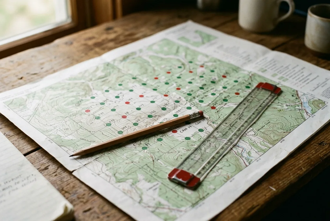
- Place cameras randomly with respect to animal movement. Use a random or systematic-with-random-origin design. Nudging a camera a few metres to reach a tree is fine; deliberately choosing a trail, scrape, wallow, or bait is fatal to an unbiased estimate.
- Use high-performance cameras. Fast trigger (well under a second), reliable recovery, and either video or rapid image bursts. Slow or flaky triggers undermine the "certain detection" assumption at the heart of REM, REST, CT-DS, and TTE alike.
For effort, the brute arithmetic is sobering but useful. The encounter rate between cameras dominates the variance, so more camera locations beats longer deployments at fewer locations. Concrete CT-DS targets from a large effort-versus-precision study: a coefficient of variation around 20% needs roughly 100 sampling days at 50 locations, or 100 to 150 locations for a shorter survey; pushing to a CV of 10% can require more than 200 locations. Plan accordingly, and be honest with yourself before you start about whether your target species is common enough to reach usable precision at all.
On the software side, the good news is that the tooling is open and improving. Density estimation in R is well supported — there's a maintained walkthrough covering REM, time-to-event and space-to-event, N-mixture, and unmarked spatial capture-recapture — and the activity correction lives in the `activity` package, while distance sampling has program Distance behind it. The same R-focused chapter is refreshingly candid that estimating density from camera data "is not easy, often isn't precise," and usually means real work — a healthy attitude to carry in.
The frontier is automation, and it's arriving fast. A semi-automated CT-DS workflow now uses a deep-learning depth model plus an automated animal detector to measure observation distances straight from photos, calibrated with just two reference images per camera. It produced density estimates statistically indistinguishable from painstaking manual measurement while cutting data-processing time more than thirteenfold — collapsing weeks of distance annotation into a couple of days. Multi-species methods are advancing too: a Bayesian extension of REM now estimates density for an entire community at once, including the rarest species, using only information pulled from the images themselves.

The bottom line
There is no universal method, and anyone who tells you otherwise is selling something. REM, CT-DS, REST, TIFC, and the time-to-event family are all legitimate, all peer-reviewed, and all capable of producing density estimates that hold up against independent surveys — when their assumptions are respected. Choose by your species' behaviour and your data realities, not by which method has the prettiest derivation. Respect random placement above all. Measure your detection zone. Check the activity assumption. And size your survey for the precision you actually need, knowing that for rare species, the answer might still be "you can't get there from here without marks". Used with that clear-eyed humility, cameras turn a pile of unattributable photos into one of the most powerful, least invasive density tools wildlife science has.
Frequently asked questions
Can you really estimate animal density from a camera trap without identifying individuals?
Yes — that's exactly what methods like the Random Encounter Model, camera-trap distance sampling, REST, TIFC, and space-to-event were built to do. They convert detection rate into animals per km² by correcting for detectability and movement instead of counting recognizable individuals. Validation studies show they match independent estimates well for common-to-moderately-rare species, though usually with less precision than capture-recapture.
What's the difference between the Random Encounter Model and distance sampling for cameras?
REM models animals like colliding gas particles and needs an estimate of how far they travel per day, which is its main weakness. Camera-trap distance sampling instead measures the distance to each animal at fixed snapshot moments and models how detection falls off with distance — so it never needs a movement-speed estimate, but it does require certain detection right in front of the camera.
Why can't I just put cameras on game trails to get more photos?
Because every unmarked-density method assumes cameras are placed randomly with respect to where animals go. Targeting trails, scrapes, water, or bait concentrates detections in non-representative spots and biases the density estimate — sometimes drastically. A Random Encounter Model study underestimated one species by 86% from biased placement, and an elk study overestimated by 116% partly from game-trail cameras.
How many cameras do I need for a reliable density estimate?
More than most people expect. Because variation between camera locations dominates the uncertainty, you generally want 100 or more locations to reach a coefficient of variation under 20% — the threshold for detecting real population change. Adding locations helps more than running fewer cameras for longer. For genuinely rare species, even an ambitious survey may not reach usable precision.
Which method handles rare species best, and which is best for abundance?
For abundant species, REST tends to give the best precision for the least effort; for sparse populations, camera-trap distance sampling squeezes more out of each detection. But for genuinely rare animals, all the unmarked methods struggle — one validation study found they failed for jaguars while working for the more common species alongside them — and spatial capture-recapture (if the animals are identifiable) is the better bet.
Do I need video, or will still images work?
It depends on the method. REST works best with video to measure staying time; TIFC and the time-to-event methods can use still images or time-lapse. One important catch for still-image distance sampling: you must account for the camera's recovery time and retrigger delays when calculating survey effort, or you can underestimate density by up to 96%.